Human Readable Magazine

The use of the right data structure that is adequately suited for the complexity of a problem is one of the attributes that distinguishes experienced developers from the rest.
After several years of plying my trade as a software engineer, I assumed I had at least encountered most of the consequential data structures in the field.
Unfortunately, important fundamental techniques do not always make it into the mainstream of computer science education.

Suffix trees, primarily used for indexing and searching strings, occupy a central position in text compression, text algorithmics, and applications in the realm of biological sequence comparison, and motif discovery.
This data structure had never been on my radar until fairly recently when a job interview confronted me with its existence.
Several culprits are to blame for its relative anonymity.

Introduced to the world in 1973 by Peter Weiner, suffix trees are a relatively new concept in computer science, with this newness likely fueling its obscurity.
In addition, a suffix tree first needs to be built, and its construction algorithms are nontrivial. At the time of this writing, there aren’t any Java or other language libraries that provide the necessary functions.
This degree of difficulty in its implementation presumably limits its widespread usage. Moreover, because even the image of a suffix tree looks complicated at first sight, some people might be intimidated and discouraged from learning it. Furthermore, it is one of those few data structures developed to solve a super specific problem, which somewhat adds to the sheen of the suffix tree being in a class of its own.

However, regardless of the underlying reasons, suffix trees are perhaps the most important data structures for string processing but have flown under the radar for far too long.
To the extent it can, this article hopes to remedy this problem while attempting to demystify the suffix tree’s inner workings. This juggling act is a tall order, but I am hoping to validate the cliché that it is better to shoot for the moon and miss in the hope of landing, at the very least, among the stars.

The Problem, the Suffix Tree, and Ukkonen’s Algorithm

A suffix tree is a compressed trie of all the suffixes of a given text as keys, with their positions within the text as values. The trie will be elaborated upon in a subsequent section, but in the meantime, in order to grasp an intuitive understanding of the suffix tree, it is better to view it from the perspective of the problem it was intended to address.

The fountainhead, the patient zero, if you will, for the compelling suffix tree remedy is the substring problem. This challenge, expressed in various forms in computer science literature, boils down to finding the means to preliminary process a text in such a way that this computational string matching problem is solved in time proportional to the length of the pattern. The problem has many more applications than its face value would suggest. The most compelling is performing intensive queries on a large database, represented by $T$ .

The prototypical problem for a suffix tree can be expressed more technically as follows: Given a particular string $T$ , we need to construct an efficient data structure $S$ , such that $S$ will serve as an index of $T$ , enabling us to efficiently query text $T$ for all the occurrences of a query pattern $P$ .
Therefore, the foremost benefit of a suffix tree is to enhance pattern matching on an indexed string.
The challenge, however, is to index the text $T$ in such a way that given a query pattern $P$ , all the occurrences of $P$ in $T$ can be reported efficiently. In case you haven’t already inferred it, a suffix tree is the data structure $S$ that can meet this requirement.

Suffix trees are used for preprocessing strings, which is simply another fancy word for indexing a string in this context. The ensuing structure it generates subsequently makes it easier to search for patterns within the string. In other words, it allows us to preprocess the string, only once, in anticipation of future, unknown queries.
Such future inquiries could be to determine whether $P$ is a substring of $T$ , how many times $P$ appears in $T$ , the longest repeated string in $T$ , the longest common substring of $P$ and $T$ , just to mention a few of the enticing possibilities.

However, the suffix tree is not a pattern-matching algorithm. Such distinction is reserved for algorithms such as Knuth-Morris-Pratt (KMP), Boyer-Moore, and Rabin Karp, among others. As a result, this article will fixate on the construction of the suffix tree; any mention of how pattern searching can be implemented through it is regarded as an ancillary benefit.

One of the true geniuses of the suffix tree is how it allows different kinds of queries to be answered quickly, permitting its use as a particularly fast implementation of many important string operations.
But the hardest part is constructing the tree. If you use the naïve algorithm, constructing a suffix tree for a string of size $n$ takes $O(n^2)$ time, which is clearly prohibitive.

However, by virtue of the fact that all the entries of its tree are suffixes of the same string, they share a lot of information that can be exploited for efficiency. Consequently, algorithms that take advantage of this commonality allow us to create the suffix tree more proficiently.
For instance, by using Ukkonen’s algorithm, a suffix tree can be built in linear time and space. Ukkonen’s algorithm stands out because most algorithms that either construct an index or query for a pattern lack the generous running time and memory savings that it does.

To paint the Ukkonen’s algorithm savings in asymptotic terms, assuming $n$ is the length of $T$ and $m$ is the length of $P$ , then the construction time and space complexity of the suffix tree are both $O(n)$ , which allows the given query string (pattern) $P$ of length m to be queried in $O(m)$ time.
This is in sharp contrast to other algorithms, which may take up to $O(n+m)$ time, rendering them prohibitively inefficient to use, especially with large databases.
This means that someone could determine whether the term "banana" was in the entire collection of Encyclopedia Britannica just by performing seven character comparisons!

Ukkonen’s algorithm has several important attributes and innovations that enable it to deliver these linear time and space advantages. These are simple features, yet they exert a disproportionate impact on its overall performance.

First, it is online, which simply means it processes the string symbols one character at a time, from left to right. This allows the index to always have the tree for the scanned part of string already ready. Imagine the algorithm is about to add a character at say, position $4$ in the string. This means it already has the tree $T_3$ built from suffixes $0$ to $3$ . This capability in the tree-building phase opens the door to another remarkable feature known as the suffix link.
We will see how the suffix link operates later on, but at this point, it suffices to say that it enables the build process to shorten its migration path when required to move from one branch/node to another. This is necessary because Ukkonen’s algorithm computes its suffix tree from another data structure, albeit a similar one, known as an implicit suffix tree. Implicit suffix trees do not deliver linear complexity when computed in a straightforward manner, hence the need for suffix links to speed up tree traversal. In addition, these suffix links are convenient for pattern matching after the tree has been constructed.

To wring space savings from the suffix tree, instead of storing single characters in its edge labels, Ukkonen labeled them as a pair of integer pointers to the text. This edge uses O(1) space, even though it carries a string of arbitrary length. As a result, this edge-label compression leads to memory space reduction.

Another interesting feature of the suffix tree is the manner in which it exposes the internal structure of a string and, by so doing, provides an ease of access into it. This thread of thought is a good way to segue into unveiling the properties of the suffix tree:

A suffix tree of string $S$ and length $n$ is defined by the following characteristics:
	* Its leaf nodes will correspond exactly to its length $n$, numbered $1$ to $n$.
	* Apart from its root, every other internal node has at least two children.
	* Every edge is labeled with a non-empty substring of $S$.
	* Two edges with a common node cannot have string-labels starting with the same character.
	* The resultant string obtained by concatenating all the labels found on the path from the root to leaf *i* spells out suffix S[i..m], for i=1,…, s.

Understanding the Suffix Tree from the Perspective of a Trie

A suffix tree is built on top of a trie, so it is necessary to have some rudimentary understanding of the trie.
In an overly simplified manner, the prefix and suffix distinction can serve as a mnemonic device to differentiate between a trie and a suffix tree, which is to remember that the latter deals with suffixes while the former, prefixes. Obviously, their overall differences aren’t that simplistic.

A trie is simply a tree for storing (a set of) strings $S$ , in which there is one node for every common prefix. The path from the root of the trie to any of its nodes corresponds to a prefix of at least one string of $S$ . In addition, the strings that are in the set $S$ are stored in extra leaf nodes. A suffix tree, on the other hand, is an improvement and a more compact representation of the trie because not every trie node is explicitly represented in the tree. It corresponds to the suffixes of a given string where all nodes with one child are merged with their parent. So instead of just adding the text itself into the trie, every possible suffix of that text is added.

The trie's edge labels are in actual characters, unlike the suffix tree (Ukkonen’s implementation at least), which uses numeric pointers to conserve space.
Since the suffix tree removes the unnecessary branches of the trie, it consequently doesn’t require as much space. As a result, it is lighter than the trie and has innovations such as suffix links that make it equally faster.

The lightness and speed advantage over the trie enables the suffix tree to be used to index DNA or optimize some large web search engines.
Their differences also inform the type of use cases in which they are utilized and the questions demanded of them in queries, even where some large text is given.

Since tries store a set of strings, they can be used to search for predefined words in a text, like ensuring users do not post derogatory words by building a trie containing those forbidden, predefined words.
Conversely, a suffix tree can be built to search for any words in the text. Most of us who have used the CTRL+F search feature in any text editor will appreciate this benefit function.
For this hypothetical large text, once it is changed or modified in any form, you’ll also be compelled to rebuild both the trie and suffix tree. Doing so for the trie is a relative trivial operation. But both the building and rebuilding of a suffix tree for a large amount of text is a complex operation.

A Suffix Tree for BANANA$

We will use BANANA$ as the text to understand how suffix trees are built. In order to avoid an implicit suffix tree and ensure suffixes end at leaves, we add $ char at the end of the string. The termination character can be any that isn’t in the alphabet the string is taken from. Following are all the possible suffixes of BANANA$:

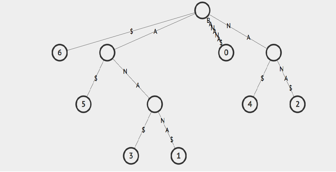
Fig. 1: Suffix Tree for BANANA$

Starting from the root node, each of the suffixes of BANANA$ can be found in the tree (BANANA$(0), ANANA$(1), NANA$(2) …) and finishing up with a solitary $ at index 6. Because of this organization, you can search for any substring of the word by starting at the root and following matches down the tree until exhausted.

The key feature of the suffix tree is that for any leaf $i$ , the concatenation of the edge-labels on the path from the root to leaf $i$ will spell out the suffix of $S$ , which starts at the position $i$ .

Suffix Tree and Its Construction

The general approach to building a suffix tree is twofold:

Generate all the suffixes for that text.
Take all the suffixes as individual words and build a compressed trie with them.

Components of Suffix Tree

Being a tree data structure, a suffix tree is comprised of a root and internal and leaf nodes. This article only elaborates on those components and areas that have particular significance in the operations of a suffix tree.

Edges: A suffix tree of a string $S$ represents all the suffixes of the string. Each edge of the suffix tree is labeled with a substring $y$ of $S$ , and the edge string $y$ is represented by a pair $(i, j)$ of positions such that the substring of $S$ that begins at position $i$ and ends at position $j$ is identical to $y$ .
Therefore, the pair $(i, j)$ are essentially pointers to the text, enabling the edges to carry string labels of arbitrary length. This ensures a suffix tree can be represented with linear space since the pointers take only $O(1)$ space.

If the edge labels were stored as strings, space complexity would be $O(N^2)$ , regardless of the number of nodes. Using two variables $(i, j)$ as edge labels instead of strings takes constant space, making overall space complexity $O(1)$ .

Internal Nodes: They have more than one outgoing edge and mark the parts of the tree where branching occurs. Branching only occurs whenever a repeating string is involved.

Suffix Link: In order to achieve linear time both in its construction algorithms and the many applications that utilize it, the internal nodes of suffix trees are equipped with a suffix link. The suffix link is an important piece of acceleration. Suffix links are auxiliary edges, which occur whenever two nodes share the same substring except for the first character.

Assume there is a string $S$ in a tree, and its path from the root ends in a node $x$ . If another string &S also present in the tree (where & is any character), and its path from the root ends in node y, then the link from x to y is known as a suffix link.
Therefore, every internal node x that has a label from the root to x of more than one character must have a suffix link to exactly one other internal node.

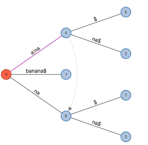
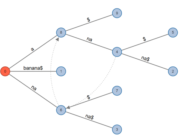
Fig. 2: Suffix Links for BANANA$

The dotted lines in Fig 2 show the suffix links from ana to na, and na to a.

Suffix tree constructions based on suffix links have gained popularity because they are simple, easy to implement, can operate online in linear time, and are conveniently suited for pattern matching.
Suffix links are not part of the suffix tree definition and therefore not required. However, they assist in a surprising number of ways. For instance, after inserting the final character of a suffix S at a node x, the algorithm will need to insert the final character of suffix S-1 in $O(1)$ time. To accomplish this, it uses the suffix link to jump right to $x^-1$ to make the insertion. This reduces the number of branch lookup operations.

Active Point: This is the point where traversal begins in any extension. It is the location identified by a point on an edge in the tree and comprises the active node, active edge, and active length. Each extension will get the active point set correctly by the previous extension. This location is found by specifying a node, an edge from that node (by identifying the first character), and a length along that edge.

Remainder: It signals the number of suffixes that must be explicitly added. In our BANANA example, if the remainder is 3, then the last three suffixes (ANA, NA, A) must be processed.

Global End: When a node is added, it automatically becomes a leaf node. Therefore, the edge to the leaf node will have the actual end of the inserted string. As a result, the algorithm assigns a global end to the edge, and this needs incrementing each time the next character is processed, making these edges grow longer automatically.

Implementation Details

Ukkonen’s algorithm constructs from a given string of text T, an implicit suffix tree Ti for each prefix S[l ..i] of S. It starts with an empty tree, then progressively adds each of the n prefixes (where length of input text is n) of T to the suffix tree.

Very High-Level Overview of Ukkonen’s Algorithm

Generate I11. Keep generating Ii+1 from Ii1. At the last stage when the terminal symbol $ is added, the implicit suffix tree will automatically be converted to a true suffix tree.

High-Level Overview of Ukkonen’s Algorithm (Pseudocode)

Finally, the true suffix tree for S is built from Tm by adding $.

Build Tree
1. For i from 1 to m - 1 do
/* begin {phase i + 1} */
     2. For j from 1 to i + 1
     /* begin {extension j} */
     3. Locate the end of the path from the root labeled S[j..i] in the current tree.
     If needed, extend that path by adding character S(i + l),
     therefore ensuring that string S[j..i + 1] is in the tree.
    /* end {extension j} */
/* end {phase i + 1} */

Phases and Extensions Decoded

Ukkonen’s method utilizes an online algorithm, so all characters are processed singularly in sequence (as evidenced by the outer loop iteration), and time taken to build the suffix tree is $O(m)$ .

 1. For i from 1 to m - 1 do

This is the tree-building phase, where tree Ti+1 is built from tree Ti. The algorithm builds from left to right, starting with the first character: $T_1$ using the first character, $T_2$ using the second character, $T_3$ using the third character, … , $T_m$ using the mth character.
Every phase i+1 is further divided into i+1 extensions, one for each of the i+1 suffixes of $S[1..i+1]$ .

Suffix Extension

Each phase deals in sequence with one character from the string, subsequently performing "extensions" within that “phase” to add suffixes that begin with the character.
This is helpful because of the repeating substructure of suffix trees, whereby each subtree can appear again as part of a smaller suffix.

 2. For j from 1 to i + 1

In the inner loop, an attempt is made to locate the end of the path $S[j..i]$ from the root. A suffix extension is performed based on the result of the previous step by adding the character $S(i+1)$ to its end (if it is not there already).

So in the case of BANANA$, for phase 4 which is building on tree $T_3$ (suffixes: BAN, AN, NA), the extensions part of the algorithm $S[1..4]$ would subsequently yield these suffixes: BANA, ANA, NA, and A because of adding S(4), which is the character A.

 3. Locate the end of the path from the root labeled $S[j..i]$ in the current tree.

While suffix extensions are based on adding the next character to the suffix tree built so far, there are certain rules governing these extensions:

Rule 1

This rule can be summarized as follows: Assuming the path from the root labeled S[j..i] ends at a leaf edge (S[i] is the last character on leaf edge) then character S[i+1] is just added to the end of the label on that leaf edge.
In extension j of phase i+1, the algorithm first finds the end of the path from the root labeled with substring $S[j..<(i+1)]$ , which is depicted in line number 3 of our pseudocode.
It then extends the substring by adding the character S(i+1) to its end (if it is not there already).
For example, in extension 1 of phase i+1, we put string S[1..i+1] in the tree. Note that S[1..i] will already be present in the tree due to previous phase i, so the algorithm just needs to add S[i+1]th character in tree, assuming it isn’t already there.

Rule 2

Assuming the path from the root labeled S[j..i] ends at a non-leaf edge (character(s) exist after S[i] on the path) and the next character is not s[i+1], then a new leaf edge with the label s[i+1] and number j is created starting from character S[i+1].
A new internal node will also be created if s[1..i] ends inside (in-between) a non-leaf edge.

Rule 3

Assuming the path from the root labeled S[j..i] ends at a non-leaf edge (characters exist after S[i] on the path) and next character s[i+1] is already in the tree, do nothing.

Illustration of Suffix Tree Construction Using Ukkonen’s Algorithm

Phase 1. This will read the first character from the string, will go through 1 extension.

Active Point=>b: Look from root. Add to root.

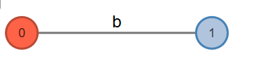
Fig. 3: Active Node: 0, Active Edge: Null, Active Length: 0, Remainder: 0

Rule 2. Extension 1 will add the suffix "b" into the tree. Creates a leaf edge b. Phase 1 completes here.

Phase 2. This will read the second character; will go through at least one and at most two extensions.

Active Point=>a: Look from root. Add to root.

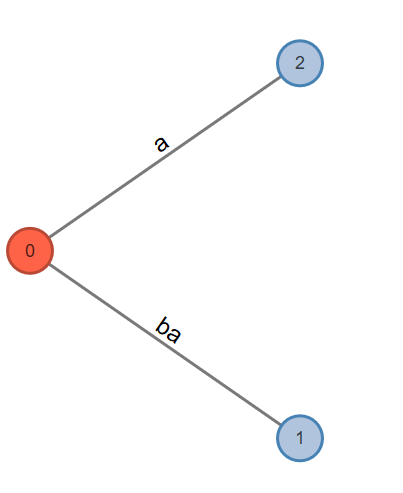
Fig. 4: Active Node: 0, Active Edge: Null, Active Length: 0, Remainder: 0

Rule 1. Extension 1 adds the suffix "ba" into the tree. Extends leaf edge from b to ba. Phase 2 extension 1 completes.

Rule 2. Extension 2 adds the suffix "a" into the tree. Creates a leaf edge a. Phase 2 extension 2 completes here.

Phase 3. This will read the third character and will go through at least one and at most three extensions.

Active Point=>n: Look from root. Add to root.

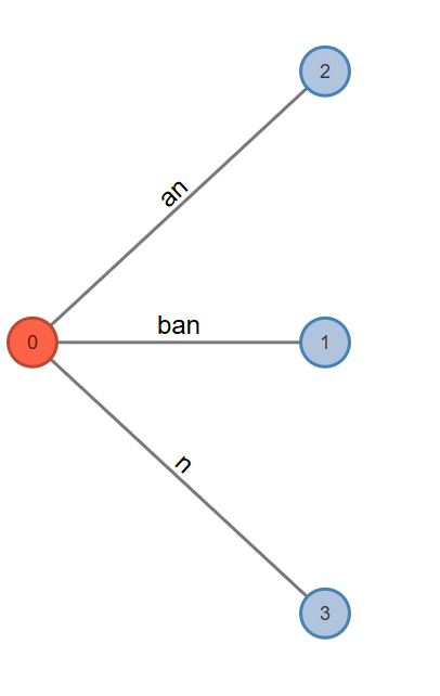
Fig. 5: Active Node: 0, Active Edge: Null, Active Length: 0, Remainder: 0

Rule 1. Extension 1 adds suffix "ban" into the tree. Extends leaf edge from ba to ban. Phase 3 extension 1 completes.

Rule 1. Extension 2 adds suffix "an" into the tree. Extends leaf edge from a to an. Phase 3 extension 2 completes.

Rule 2. Extension 3 adds suffix "n" into the tree. But there is no path from root, going out with label ’n’, so create a leaf edge n. Phase 3 extension 3 completes here.

Phase 4. This will read the fourth character and will go through at least one and at most four extensions.

Active Point=>a: Look from root. Find it ("ana"). Set it as the active point.

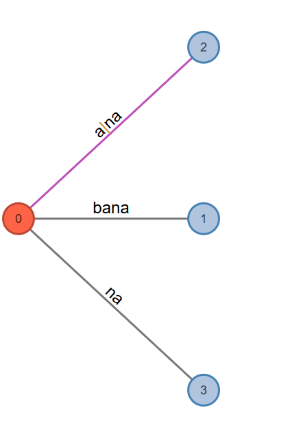
Fig. 6: Active Node: 0, Active Edge: a, Active Length: 1, Remainder: 1

Rule 1. Extension 1 adds the suffix "bana" into the tree. Extends leaf edge from ban to bana. Phase 4 extension 1 completes.

Rule 1. Extension 2 adds the suffix "ana" into the tree. Extends leaf edge from an to ana. Phase 4 extension 2 completes.

Rule 2. Extension 3 adds the suffix "na" into the tree. Extends leaf edge from n to na. Phase 4 extension 3 completes.

Rule 3. Extension 4, adds the suffix "a" into the tree, but path for label ‘a’ already exists in the tree. Therefore, no more work needed and phase 4 ends here.

Phase 5. This will read the fifth character and will go through at least 1 and at most 5 extensions.

Active Point=>n: Look from previously found "a", in “_a_na”. Find it. Set it as the active point.

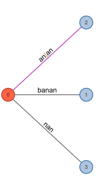
Fig. 7: Active Node: 0, Active Edge: a, Active Length: 2, Remainder: 2

Rule 1. Extension 1 adds the suffix "banan" into the tree. Extends leaf edge from bana to banan. Phase 5 extension 1 completes.

Rule 1. Extension 2 adds the suffix "anan" into the tree. Extends leaf edge from ana to anan. Phase 5 extension 2 completes.

Rule 2. Extension 3 adds the suffix "nan" into tree. Extends leaf edge from na to nan. Phase 5 extension 3 completes.

Rule 3. Extension 4, adds the suffix "an" into the tree but path for label ‘an’ already exists in the tree. Therefore, no more work needed and phase 5 ends here.

Phase 6. This will read the sixth character and will go through at least one and at most six extensions.

Active Point=>a: Look from previously found "n" in “a_n_an”. Find it. Set it as the active point.

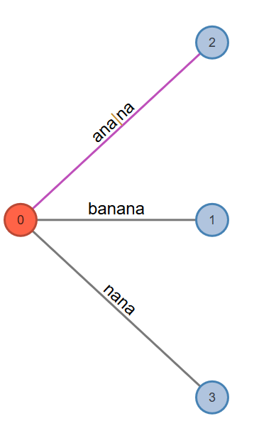
Fig. 8: Active Node: 0, Active Edge: a, Active Length: 3, Remainder: 3

Rule 1. Extension 1 adds the suffix "banana" into the tree. Extends leaf edge from banan to banana. Phase 6 extension 1 completes.

Rule 1. Extension 2 adds the suffix "anana" into the tree. Extends leaf edge from anan to anana. Phase 6 extension 2 completes.

Rule 2. Extension 3 adds the suffix "nana" into the tree. Extends leaf edge from nan to nana. Phase 6 extension 3 completes.

Rule 3. Extension 4, adds the suffix "ana" into the tree, but path for label ‘ana’ already exists in the tree. Therefore, no more work needed and phase 6 ends here.

Phase 7. This will read the seventh character and will go through at least one and at most seven extensions. Active Point=>$: Look from previously found "a" in “an_a_na”. This is not found, so add an internal node and add $. Then change the active point to the same character in a smaller (suffix) edge: “a” in “n_ana”.

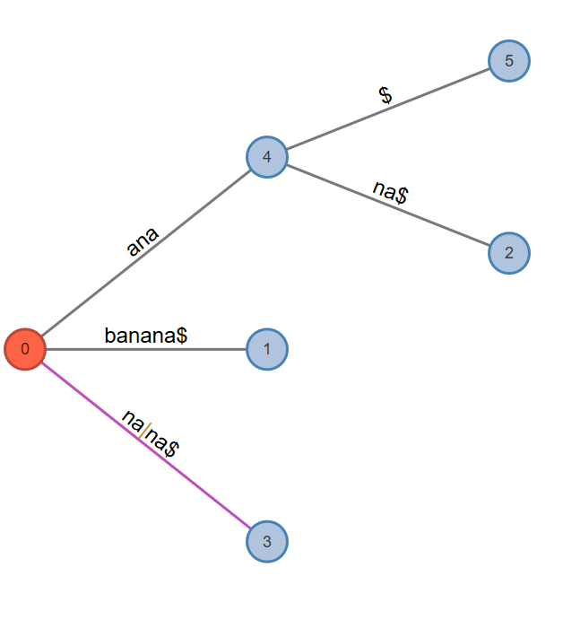
Fig. 9: Active Node: 0, Active Edge: n, Active Length: 2, Remainder: 2

Rule 1. Extension 1 adds the suffix "banana$" into the tree. Extends leaf edge from banana to banana$. Phase 7 extension 1 completes.

Rule 1. Extension 2 adds the suffix "anana$" into the tree. Extends leaf edge from anana to anana$. Phase 7 extension 2 completes.

Rule 1. Extension 3 adds the suffix "nana$" into the tree. Extends leaf edge from nana to nana$. Phase 7 extension 3 completes.

Rule 2. Extension 4 adds the suffix "ana$" into the tree, but path for label ‘ana$’ already exists in the tree on the edge now labeled “anana$”. Therefore, the algorithm splits that edge after the matching portion “ana” by adding a new internal node which contains the unmatched portion “na$” and an edge labeled with $ as a leaf node.
This represents quite the leap from what has been previously done, so let’s summarize: There’s an edge from the root that starts with "ana" ending in the middle of an edge, so we perform a split adding an internal and leaf node.

Active Point=>$: Look from previously found "a" in “n_a_na$”. This is not found, so add an internal node and add the $ as leaf node. Then change the active point to same character in a smaller (suffix) edge: “a” in “_a_na$”.

Fig. 10: Active Node: 0, Active Edge: a, Active Length: 1, Remainder: 1

Rule 2. Extension 5 adds suffix "na$" in tree but path for label ‘na$’ already exists in the tree on edge now labeled “nana$”. Just as done previously, that edge is split after the matching portion “na” is given a new internal node which has an edge emanating from it that contains the unmatched portion “na$”, along with a $ pointing to a leaf node.

Active Point=>$: Look from "a" in “_a_na$”. This is not found, so add an internal node and add the $. Then change the active point to root.

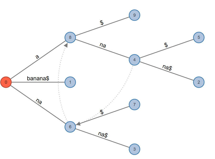
Fig. 11: Active Node: 0, Active Edge: none, Active Length: 0, Remainder: 0

Rule 2. Extension 6 adds the suffix "a$" on the path for label “ana”. The edge is split after the matching portion “ana” is given a new internal node which has an edge emanating from it that contains the unmatched portion “na”, along with another edge $ pointing to a leaf node.

Active Point=>$: Look from the root. Add to the root.

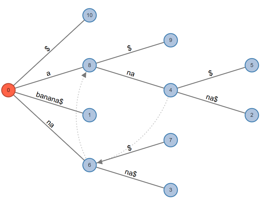
Fig. 12: Active Node: 0, Active Edge: none, Active Length: 0, Remainder: 0

Rule 2. Extension 6 adds edge labeled "$" to the root.
Our suffix tree for BANANA$ is completed.

Pattern Searching with Suffix Tree

Constructing the suffix tree is a means to an end. The purpose of the structure is to be able to make inquiries that would yield insights into a body of text (especially a large one) that would have otherwise been quite onerous to obtain.

While the scope of this article is limited to building a suffix tree, pursuing pattern searching with the structure created is not as big of a leap as one would assume. The architecture of the suffix tree provides a blueprint from which it is easy to pursue answers. For instance, the leaves below a node store the suffix indices that start with the prefix defined at that node. Because of this, you just need to count the descendant leaves after you find the node that matches your search pattern in the suffix tree.
Following are some possible queries to a suffix tree and the likely paths to follow in order to address them:

Is k is a substring of T?
Follow the path k starting from the root. If you exhaust the query string, then k is in T.

Is k a suffix of T?
Follow the path k starting from the root. If you end at a leaf at the end of k, then k is a suffix of T.

How many times does k occur in T?
Follow the path k starting from the root. The subsequent number of leaves under the node you end up in is the number of occurrences of k.

What is the longest repeat in T?
Just find the deepest node that has at least two leaves under it.

What is the first suffix alphabetically?
From the root, follow the edge label with the alphabetically smallest letter.

These are obviously simplified suffix tree procedures, but just like the axiom that holds that personnel is policy, the structure is the solution—or at least provides a road map to the solutions.

Conclusion

Suffix trees are useful in various cutting-edge applications. For developers, engineers, and data scientists, understanding its working mechanism has the potential to open up exciting vistas of opportunities, especially in areas such as bioinformatics and computational biology.

I hope that this article, while not exhaustive of the subject, was able to shed light on suffix trees' importance.

Bibliography

Cazaux, Bastien and Rivals, Eric. "Reverse Engineering of Compact Suffix Trees and Links: A Novel Algorithm." Journal of Discrete Algorithms 12 (2014): 9–22. Accessed December 4, 2017. https://www.sciencedirect.com/science/article/pii/S157086671400046X.

Gusfield, Dan. "Algorithms on Strings, Trees, and Sequences." University of California, Davis. (1997). https://web.stanford.edu/~mjkay/gusfield.pdf

Larsson, N. Jesper, Fuglsang, Kasper and Karlsson, Kenneth. "Efficient Representation for Online Suffix Tree Construction." IT University of Copenhagen, Denmark. (2014) https://arxiv.org/pdf/1403.0457.pdf

Singh, Anurag. "Ukkonen’s Suffix Tree Construction – Part 1." https://www.geeksforgeeks.org/ukkonens-suffix-tree-construction-part-1/

"Suffix Trees and Its Construction." (2014). https://www2.cs.duke.edu/courses/fall14/compsci260/resources/suffix.trees.in.detail.pdf

Ukkonen, E. "On-Line Construction of Suffix Trees." Algorithmica 14, no. 249 (1995). https://doi.org/10.1007/BF01206331

Valentini, Edward. "Suffix Trees and Ukkonen’s Algorithm in Swift Part 1." (2017). https://edwardvalentini.com/2017/12/10/suffix-trees-and-ukkonens-algorithm-in-swift-part-1/

The Wonders of the Suffix Tree through the Lens of Ukkonen’s Algorithm